Sharing knowledgeFrom biology to models
Understand a population, then model it.
1
What is a population?
All the individuals of one species that live in the same place and can breed with one another.
The flies of an orchard, the fish of a lake: we count them, sort them by sex (females, males) and by life stage (juveniles, adults), and follow how these numbers change.
In biological control, the population to follow is the pest's. The question becomes: how can its numbers be brought down, and kept down?
2
How does a population change?
Births, deaths, and an environment that eventually limits growth.
When resources are plentiful, each individual has on average the same number of offspring, whatever the size of the population: the larger it is, the faster it grows. Then space and food run short, growth slows down and the numbers level off.
The logistic curve sums up this scenario with two numbers: the growth rate r (births minus deaths, per individual) and the carrying capacity K (the number of individuals the environment can support). Vary them.
Births minus deaths, per individual and per unit of time.
The number of individuals the environment can support.
3
Why model living systems?
To isolate a mechanism, and to test what cannot be tested in the field.
Nobody can release millions of insects to try every strategy, or make sterilisation imperfect on purpose. A model lets us ask “what if…?” without risk, and find the thresholds where everything tips over.
A model is not reality: it keeps what is useful for one specific question, and its conclusions hold within the limits of its assumptions.
4
How does a simulation work?
The computer moves forward in time step by step, applying the rules of the model.
At each step, it computes how many individuals are born and die during that short interval, then updates the numbers. The smaller the step, the more closely the simulation follows the exact solution.
At each step: N ← N + Δt × r N (1 − N/K).
10 computation steps. The models on this site use a more accurate scheme (fourth-order Runge-Kutta) with much smaller steps.
- Exact solution
- Step-by-step simulation
5
What is a compartmental model?
Individuals are sorted into boxes, and the model describes the flows between them.
In the residual-fertility model, three boxes are enough: the released sterile males, the wild females and the wild males. Each arrow is a term of a differential equation.
The model follows average numbers: it is quick to analyse mathematically (equilibria, thresholds), but it does not see individuals.
6
What is an individual-based model?
Each individual becomes an agent, with its own history and rules.
Here, each female keeps track of the sperm of the males she has mated with. This is essential to compare sperm-use rules that a compartmental model cannot represent.
The demonstrator below is a version of the published model scaled down fifty times: it shows how the model works, it does not replace the simulations of the article.
Sperm-use rule
Equivalent to 10,000 individuals per day at the scale of the original model.
Individual scale — females and the content of their spermatheca
Day 0: .
- fertile
- fertile + sterile
- sterile
- unmated
Population scale
- Larvae
- Females
- Wild males
7
From individual behaviour to collective dynamics
A detail in the life of each female can change the fate of the whole population.
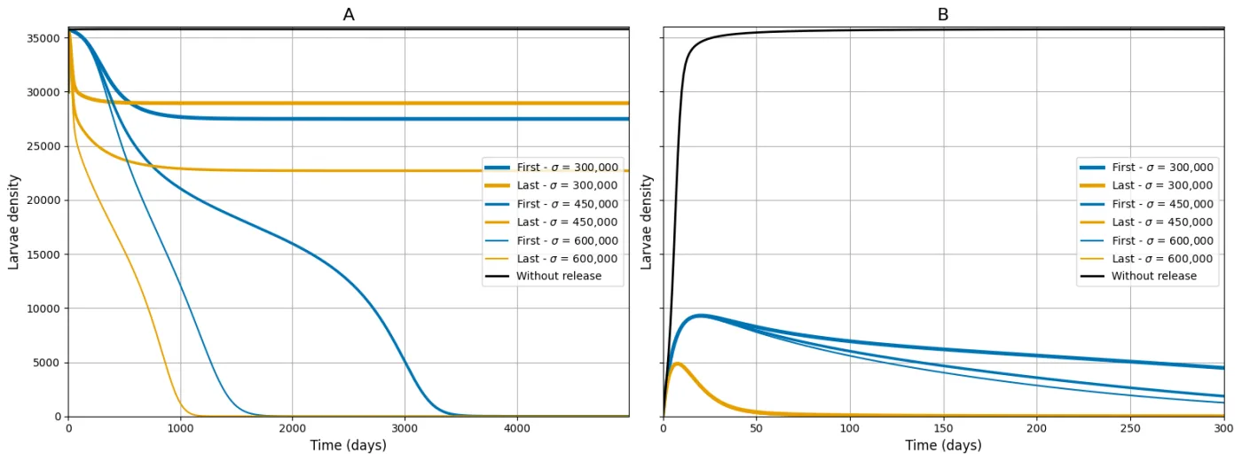
Whether females mate once or several times seems a minor detail. Yet in the 2026 article, in the long run, multiple mating calls for more releases to control the population, while in the short run it can “defertilise” females that have already mated with wild males.
This is the whole point of models: linking an individual mechanism to its effect on the population, and showing that this effect depends on the time horizon.
8
How do you interpret a result?
Look for the threshold, read the conditions, name the limits.
This diagram, redrawn from the thesis, plots the density of sterile males S present in the environment on the horizontal axis, and the equilibrium density of females F* on the vertical axis. Each curve is a possible equilibrium: solid if it is stable, dashed if it is unstable.
Below the critical value Sc, two outcomes coexist: the population persists at the stable equilibrium, or collapses if it starts too low; the unstable equilibrium acts as a threshold. Beyond Sc, only the zero equilibrium remains: the population can be eliminated.
Interpreting means stating under which conditions this threshold exists, what shifts it (residual fertility, for instance), and what the model does not say: here, the density of sterile males is assumed constant, whereas real releases make it vary.
- Stable equilibrium: the population persists at this level.
- Unstable equilibrium: it acts as a threshold; a population that starts too low collapses.
- Zero equilibrium: the population is eliminated.
- Sc, critical density of sterile males: beyond it (shaded area), only the zero equilibrium remains.
- Saddle-node bifurcation: the two equilibria meet, then vanish.