Aim
Write the biological mechanisms (competition between wild and sterile males, residual fertility, female remating) as equations, then determine for which release intensities the population is eliminated or only reduced.
Scientific value
Equations give general results rather than a series of case-by-case simulations: the existence of an elimination threshold, the conditions under which residual fertility turns suppression into mere reduction, the stability of equilibria depending on the sperm-use rule. They also serve as the reference for the individual-based model, compared with them in the appendix of the 2026 article.
Context
Most models of the sterile insect technique describe the population through average numbers (sterile males, females, wild males, larvae) whose change over time follows ordinary differential equations. This framework lends itself to mathematical analysis: equilibria, stability, thresholds.
Question
For which sterile male release intensities is a pest population eliminated, and how do residual fertility and female remating change that outcome?
Results shown
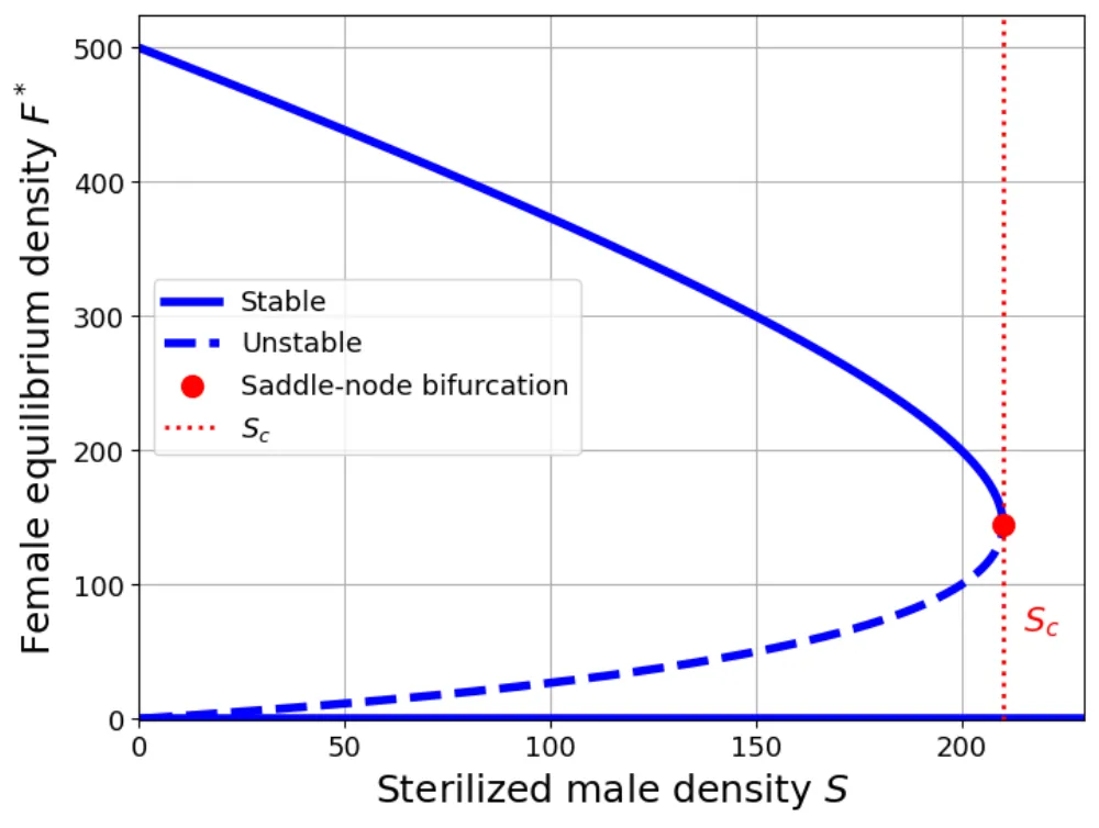
- The models separate the conditions that favour suppression of the population from those where releases mainly reduce its abundance (Bulletin of Mathematical Biology, 2025).
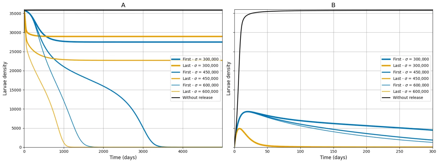
- With remating, effects differ with the time horizon: a sperm-use rule can speed up the initial decline of the population without guaranteeing its elimination in the long term (PLOS Computational Biology, 2026).
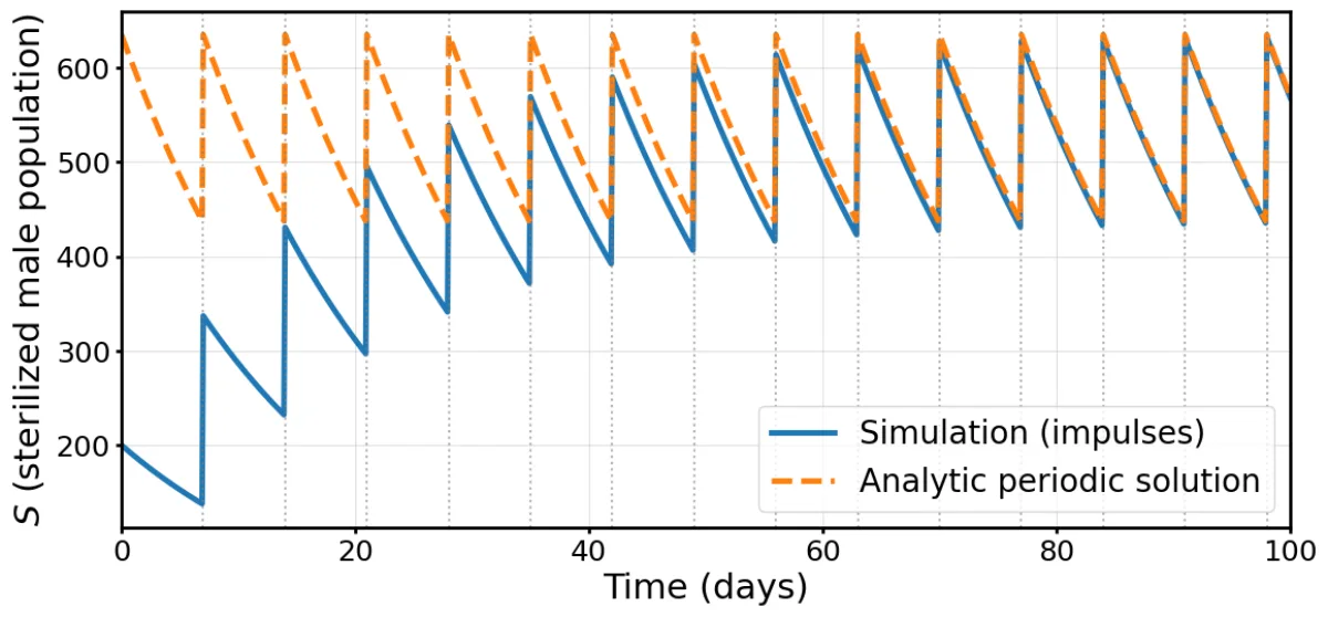
- Under a limited budget, impulsive releases reveal a trade-off between release frequency and release size (thesis, chapter 5).
Limitations
- An equation model describes average numbers: it represents neither the variability between individuals nor chance encounters, which the individual-based model handles.
- The residual-fertility model has no larval stage; the remating model adds one.
- The notebooks reproduce the published figures; they are not a software library reusable as is.
See the model at work
Observethe mechanism
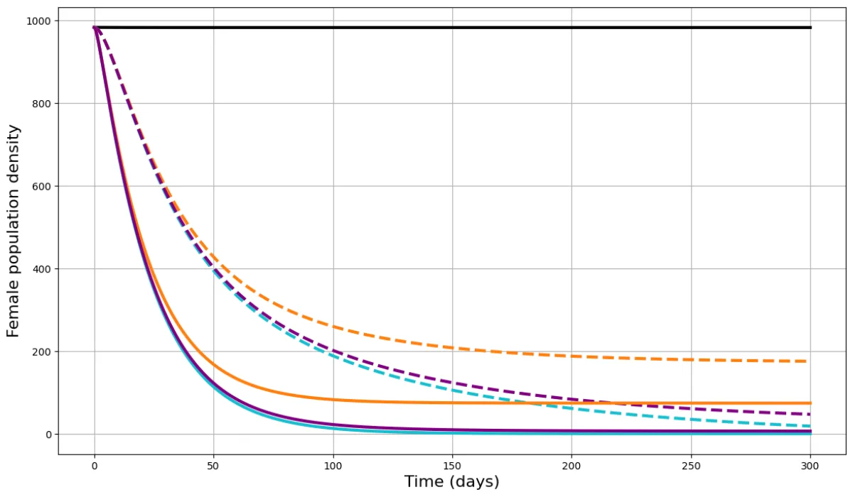
Sterilisation is not always perfect. This model follows three populations (sterile males S, wild females F and wild males M) and distinguishes two forms of residual fertility.
δ: share of released males that remain fully fertile. ε: share of matings with a sterile male that remain fertile.
Explorethe parameters
- No releases
- Releases, perfect sterility
- Releases with residual fertility
Understandthe results
At t = 300 days, the model gives 18.3 females with perfect sterility and 175.2 with residual fertility, against 983 without releases.
Raise δ: even with intense releases, the solid blue curve can settle above zero, a reduction rather than a suppression.
Courtois, Mailleret, Touzeau, van Oudenhove & Grognard (2025). Bulletin of Mathematical Biology 87, 25.
- PublicationBulletin of Mathematical Biology, 2025
- DOI10.1007/s11538-024-01401-1(new tab)
- CodeScript_Manuscrit_SIT_RF.ipynb — thesisData(new tab)
- MethodologyResearch theme: residual fertility
TypeScript port (RK4, step 0.1 day) of the notebook's modele_SIT function, with its fixed parameters and the initial condition F₀ = M₀ = 983. Checked: reproduces the notebook's “time dynamics” figure (σ = 500 and 5,000). Teaching exploration: it does not replace the published analyses.
Figures and media